Nearly 400 years ago, the mathematician Pierre de Fermat famously claimed that there are no integer solutions to the equation:

\[x^n + y^n = z^n\]

when and . [And, after centuries, this extremely difficult theorem was completely proved in 1994.]

Yet, even if there are no exact solutions to this equation, there are some striking “near misses” where the formula is almost true, for example:

$$13^5 + 16^5 = 17^5 + 12$$

$$3,472,073^7 + 4,627,011^7 = 4,710,868^7 \cdot (1 – 3.64\ldots \cdot 10^{-22})$$

In 2000, Noam Elkies published an algorithm to efficiently find these kinds of “Fermat near-misses”, based on a clever application of lattice reduction.

This post gives a sketch of that algorithm (for those of us who aren’t professional computational number-theorists) and reports some additional results that were beyond the reach of typical desktop computers twenty years ago (when the original calculations were done).

Warm-up: lattices in two dimensions

Before tackling the problem of finding near-solutions to Fermat’s equation, let’s start with a simpler problem that illustrates some of the essential ideas we’ll need: approximating

It’s well-known that is irrational, so it can’t be expressed as a ratio of two whole numbers, but there are some ratios that come close, like:

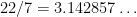
$$\pi \approx \frac{22}{7}.$$

Here’s a geometric way to think about finding good approximations of :

Consider the line , depicted here in gray:

If we can find a grid point that’s “close” to the line, then should be a good approximation to . In the mathematical jargon, we want to find a lattice point that’s close to the line. A lattice is discrete set of points of the form , where and are integers and are basis vectors for the lattice. In this example, the basis vectors are:

$$\vec{b}_1 = (1, 0)^T$$

$$\vec{b}_2 = (0, 1)^T$$

which are shown in blue in the figure, and all the gray dots are lattice points (i.e., integer combinations of these basis vectors). We’ll see other examples of lattices (and lattice bases) below.

To find points close to the line, we’ll start by encasing the line in a very skinny parallelogram (shown in orange):

The top two corners of the parallelogram have coordinates 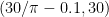and . (The bottom two corners, which are way off to the southwest of the figure, are just the negatives of these two points.) Put another way, the parallelogram is:

$$M \cdot B$$

where

$$M = \left[ \begin{matrix} 0 & 30/\pi \\ 0.1 & 30 \end{matrix}\right]$$

and is the “box” .

So, now our goal is to find the lattice points within this parallelogram of height 60 and width 0.2. To do this, we’ll invert to map the parallelogram to the box by multiplying everything by :

Now the tall, skinny parallelogram has become a nice orange square, but the lattice has gotten so stretched out that you can barely detect an angle between the blue basis vectors. Fortunately, a lattice has many different possible bases, and we can improve our situation by finding a better basis (like the one shown in red). In general, bases that are close to orthogonal are more convenient, as are bases that consist of shorter vectors – and the red basis wins on both counts: its vectors are much shorter than the blue vectors, and the angle between them is much closer to 90 degrees. This is no coincidence, since you can show that the area of the triangle formed by joining tips of the basis vectors will be the same, regardless of which basis you choose; so as the basis gets “more orthogonal”, the vectors have to get shorter (and vice versa) in order to preserve that area.

So, how do we find the red basis? Using a lattice reduction algorithm, of course! The details of these algorithms are too much to get into here (although the 2-dimensional case is much more straightforward than in higher dimensions), but suffice it to say there are very efficient algorithms that can take a very poor basis (like the stretched-out blue basis defined by ) and return an equivalent basis with short, nearly-orthogonal columns (like the much nicer red basis above). Even though the general problem of finding short vectors in a lattice is NP-hard, these algorithms tend to work very well in practice, especially in low dimensions, which is how we’re using them here.

Armed with a “good” basis for our lattice, it’s now much easier to enumerate the lattice points in the orange box. To do this, we’re going to shift our frame of reference to the basis (which we found via lattice reduction):

$$R = \left[ \begin{matrix} 0.450\ldots & -0.028\ldots \\ 0.1 & 0.733\ldots \end{matrix}\right].$$

In particular, we can express the coordinates of the corners of the orange box in terms of the basis by multiplying them by :

So, for example, the top left corner of the orange box (i.e., the point in the standard basis) has coordinates of

$$R^{-1}\cdot (-1, 1)^T = (-2.12, 1.65),$$

in the lattice defined by , and similarly for the three other corners (see the diagram above). Now, we can observe that the -coordinate of each corner is only ever between and , so the lattice points within the box must have coordinates that are integers in the range . Likewise, the -coordinates will have to be integers in the interval . In total, there are such points that need to be considered (i.e., the lattice points in the gray parallelogram above).

We can easily iterate over these 15 points, and then multiply each by , to bring them back into our original coordinate system, which yields the following 15 solutions:

$$ (9, 28), (8, 25), (7, 22), (6, 19), (5, 16), (2, 6), (1, 3), (0, 0),\\(-1, -3), (-2, -6), (-5, -16), (-6, -19), (-7, -22), (-8, -25), (-9, -28).$$

And, as expected, each of these (except for ) gives a decent approximation of , such as and , etc.

Of course, for such a small problem we could have directly searched for these solutions and found them without all the additional lattice-reduction machinery, but such naive approaches won’t work well when the numbers get big (e.g., vs. ) or when the dimension is larger than 2…

Back to Fermat

So how can we apply these ideas to the Fermat equation? Well, the solutions to Fermat’s equation lie on a “cone” whose cross-section looks like the “circle”:

$$\left(\frac{x}{z}\right)^n + \left(\frac{y}{z}\right)^n = 1.$$

Here’s a picture of this “cone” for the case of :

And for any particular ratio , you can construct a 3-dimensional parallelogram (a “parallelepiped”), that contains the points on the cone where .

Now, just as before, the goal is to find all the integer lattice points within the parallelepiped, and that can be done in essentially the same way we did above – the main difference is that we’re now operating in three dimensions, which means: (i) we map the parallelepiped to the 3-dimensional cube , (ii) apply lattice reduction in 3 dimensions, (iii) iterate over lattice points within the cube, and then (iv) map the results back to near-solutions . Another difference, is that this now has to be done for many different parallelepipeds, each one covering a small strip of the cone.

There are many details to sort out to get a fully-functioning algorithm, but this is the essence of the approach.

Does it work?

It sure does. Noam Elkies used this algorithm over 20 years ago to find solutions for where . Those results are tabulated here.

Using more modern hardware (and a bit of software optimization/engineering), we can find even larger near-misses, such as:

$$159,596,485^5 + 215,397,418^5 \approx 224,258,037^5,$$

$$26,353,375^8 + 184,473,622^8 \approx 184,473,626^8, $$

$$4,825,644,673^4 + 4,870,155,780^4 \approx 5,765,339,686^4,$$

$$67,560,034,732^4 + 73,425,253,501^4 \approx 84,047,201,182^4$$

which have relative error of , , , and respectively.

An expanded list of near-solutions is available here.

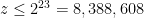
At the moment, these results cover and . As computers get faster (or as I find ways to further optimize my code) I may be able to extend the results even further.